Mostrando entradas con la etiqueta Operating System. Mostrar todas las entradas

13/3/11

Memory Translation and Segmentation

This post is the first in a series about memory and protection in Intel-compatible (x86) computers, going further down the path of how kernels work. As in the boot series, I’ll link to Linux kernel sources but give Windows examples as well (sorry, I’m ignorant about the BSDs and the Mac, but most of the discussion applies). Let me know what I screw up.

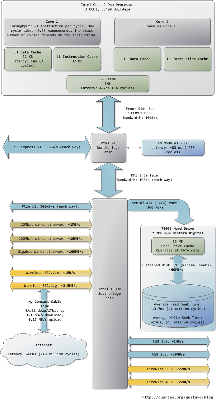
In the chipsets that power Intel motherboards, memory is accessed by the CPU via the front side bus, which connects it to the northbridge chip. The memory addresses exchanged in the front side bus are physical memory addresses, raw numbers from zero to the top of the available physical memory. These numbers are mapped to physical RAM sticks by the northbridge. Physical addresses are concrete and final – no translation, no paging, no privilege checks – you put them on the bus and that’s that. Within the CPU, however, programs use logical memory addresses, which must be translated into physical addresses before memory access can take place. Conceptually address translation looks like this:
Memory Address Translation in x86 with paging enabled
This is not a physical diagram, only a depiction of the address translation process, specifically for when the CPU has paging enabled. If you turn off paging, the output from the segmentation unit is already a physical address; in 16-bit real mode that is always the case. Translation starts when the CPU executes an instruction that refers to a memory address. The first step is translating that logic address into a linear address. But why go through this step instead of having software use linear (or physical) addresses directly? For roughly the same reason humans have an appendix whose primary function is getting infected. It’s a wrinkle of evolution. To really make sense of x86 segmentation we need to go back to 1978.

The original 8086 had 16-bit registers and its instructions used mostly 8-bit or 16-bit operands. This allowed code to work with 216 bytes, or 64K of memory, yet Intel engineers were keen on letting the CPU use more memory without expanding the size of registers and instructions. So they introduced segment registers as a means to tell the CPU which 64K chunk of memory a program’s instructions were going to work on. It was a reasonable solution: first you load a segment register, effectively saying “here, I want to work on the memory chunk starting at X”; afterwards, 16-bit memory addresses used by your code are interpreted as offsets into your chunk, or segment. There were four segment registers: one for the stack (ss), one for program code (cs), and two for data (ds, es). Most programs were small enough back then to fit their whole stack, code, and data each in a 64K segment, so segmentation was often transparent.

Nowadays segmentation is still present and is always enabled in x86 processors. Each instruction that touches memory implicitly uses a segment register. For example, a jump instruction uses the code segment register (cs) whereas a stack push instruction uses the stack segment register (ss). In most cases you can explicitly override the segment register used by an instruction. Segment registers store 16-bit segment selectors; they can be loaded directly with instructions like MOV. The sole exception is cs, which can only be changed by instructions that affect the flow of execution, like CALL or JMP. Though segmentation is always on, it works differently in real mode versus protected mode.

In real mode, such as during early boot, the segment selector is a 16-bit number specifying the physical memory address for the start of a segment. This number must somehow be scaled, otherwise it would also be limited to 64K, defeating the purpose of segmentation. For example, the CPU could use the segment selector as the 16 most significant bits of the physical memory address (by shifting it 16 bits to the left, which is equivalent to multiplying by 216). This simple rule would enable segments to address 4 gigs of memory in 64K chunks. Sadly Intel made a bizarre decision to multiply the segment selector by only 24 (or 16), which in a single stroke confined memory to about 1MB and unduly complicated translation. Here’s an example showing a jump instruction where cs contains 0×1000:
Real Mode Segmentation
Real mode segment starts range from 0 all the way to 0xFFFF0 (16 bytes short of 1 MB) in 16-byte increments. To these values you add a 16-bit offset (the logical address) between 0 and 0xFFFF. It follows that there are multiple segment/offset combinations pointing to the same memory location, and physical addresses fall above 1MB if your segment is high enough (see the infamous A20 line). Also, when writing C code in real mode a far pointer is a pointer that contains both the segment selector and the logical address, which allows it to address 1MB of memory. Far indeed. As programs started getting bigger and outgrowing 64K segments, segmentation and its strange ways complicated development for the x86 platform. This may all sound quaintly odd now but it has driven programmers into the wretched depths of madness.

In 32-bit protected mode, a segment selector is no longer a raw number, but instead it contains an index into a table of segment descriptors. The table is simply an array containing 8-byte records, where each record describes one segment and looks thus:
Segment Descriptor
There are three types of segments: code, data, and system. For brevity, only the common features in the descriptor are shown here. The base address is a 32-bit linear address pointing to the beginning of the segment, while the limit specifies how big the segment is. Adding the base address to a logical memory address yields a linear address. DPL is the descriptor privilege level; it is a number from 0 (most privileged, kernel mode) to 3 (least privileged, user mode) that controls access to the segment.

These segment descriptors are stored in two tables: the Global Descriptor Table (GDT) and the Local Descriptor Table (LDT). Each CPU (or core) in a computer contains a register called gdtr which stores the linear memory address of the first byte in the GDT. To choose a segment, you must load a segment register with a segment selector in the following format:
Segment Selector
The TI bit is 0 for the GDT and 1 for the LDT, while the index specifies the desired segment selector within the table. We’ll deal with RPL, Requested Privilege Level, later on. Now, come to think of it, when the CPU is in 32-bit mode registers and instructions can address the entire linear address space anyway, so there’s really no need to give them a push with a base address or other shenanigan. So why not set the base address to zero and let logical addresses coincide with linear addresses? Intel docs call this “flat model” and it’s exactly what modern x86 kernels do (they use the basic flat model, specifically). Basic flat model is equivalent to disabling segmentation when it comes to translating memory addresses. So in all its glory, here’s the jump example running in 32-bit protected mode, with real-world values for a Linux user-mode app:
Protected Mode Segmentation
The contents of a segment descriptor are cached once they are accessed, so there’s no need to actually read the GDT in subsequent accesses, which would kill performance. Each segment register has a hidden part to store the cached descriptor that corresponds to its segment selector. For more details, including more info on the LDT, see chapter 3 of the Intel System Programming Guide Volume 3a. Volumes 2a and 2b, which cover every x86 instruction, also shed light on the various types of x86 addressing operands – 16-bit, 16-bit with segment selector (which can be used by far pointers), 32-bit, etc.

In Linux, only 3 segment descriptors are used during boot. They are defined with the GDT_ENTRY macro and stored in the boot_gdt array. Two of the segments are flat, addressing the entire 32-bit space: a code segment loaded into cs and a data segment loaded into the other segment registers. The third segment is a system segment called the Task State Segment. After boot, each CPU has its own copy of the GDT. They are all nearly identical, but a few entries change depending on the running process. You can see the layout of the Linux GDT in segment.h and its instantiation is here. There are four primary GDT entries: two flat ones for code and data in kernel mode, and another two for user mode. When looking at the Linux GDT, notice the holes inserted on purpose to align data with CPU cache lines – an artifact of the von Neumann bottleneck that has become a plague. Finally, the classic “Segmentation fault” Unix error message is not due to x86-style segments, but rather invalid memory addresses normally detected by the paging unit – alas, topic for an upcoming post.

Intel deftly worked around their original segmentation kludge, offering a flexible way for us to choose whether to segment or go flat. Since coinciding logical and linear addresses are simpler to handle, they became standard, such that 64-bit mode now enforces a flat linear address space. But even in flat mode segments are still crucial for x86 protection, the mechanism that defends the kernel from user-mode processes and every process from each other. It’s a dog eat dog world out there! In the next post, we’ll take a peek at protection levels and how segments implement them.

Comments
36 Responses to “Memory Translation and Segmentation”

1.Chuck on August 12th, 2008 7:03 am
For what it’s worth, I’m really enjoying your articles. Please continue to write
2.Mahesh on August 12th, 2008 9:40 pm
I liked the explanation, very well articulated.
3.Gustavo Duarte on August 13th, 2008 12:34 am
@Chuck: it’s worth a lot I enjoy writing these posts, I write them for fun but the fact that people seem to like them is definitely encouraging too.

I’m cooking up the next one here… I’m actually in Hawaii this week, I’ve been waking up at ~6am to snorkel and dive, sleeping early, but this evening I’m writing a bit of the protection stuff

@Mahesh: thanks!
4.Arvind on August 13th, 2008 2:35 am
Nice article!! I have subscribed to your blog feed and everytime I check for new items your blog is the first I look for unread items..Elated that I found one today..Good read..
5.Ben fowler on August 13th, 2008 4:53 pm
I thoroughly enjoyed this well-written article as well as your others. It’s interesting, but challenging material for a lot of people, and I know it’d otherwise take a LOT of reading around to get the information elsewhere.

You have a knack for this Gustavo! Have you considered teaching, or at least turning this material into a book? Keep up the great work!
6.notmuch on August 15th, 2008 9:08 am
Nicely done. For long I have been pondering upon how to visualize the workings of hardware. From CPU clock cycle and instructions, interrupt mechanism and interaction with software, and memory. These articles are a good step in that direction. Thanks much.
7.JinxterX on August 17th, 2008 10:48 am
You write great articles, thanks, any chance of doing one on Linux and MTRRs?
8.Hormiga Jones on August 19th, 2008 9:22 am
Your series of articles are HIGHLY informative and well written. I have forwarded them onto several of my work colleagues. Thank you for this valuable resource and keep up the good work.
9.CPU Rings, Privilege, and Protection : Gustavo Duarte on August 20th, 2008 12:39 am
[...] let’s see exactly how the CPU keeps track of the current privilege level, which involves the segment selectors from the previous post. Here they [...]
10.Gustavo Duarte on August 20th, 2008 12:51 am
Thank you all for the feedback!

I was in Hawaii last week, hence the belated reply. I did crank out the protection stuff in the flight back to Denver though

@Ben: You know, I started the blog just as a way to write random stuff. I never expected to get hits hehe. So now I have thought about some of the stuff you mentioned, especially books.

The trouble with books is that the stuff ends up locked and inaccessible to people, plus you lose things like being able to link to the source code directly (or linking in general).

I also thought about doing a print-friendly CSS or maybe render some stuff as PDF to let people download. That might be a good way to go.

Teaching would be fun… I love teaching people who are interested in learning. hehe. I don’t plan ahead too much, so I guess I’ll see where it goes. Thanks for the encouraging words.

@JinxterX: yea, that sounds cool. I thought about writing about cache lines and how memory access happens “for real”, and talking about MTRRs would make a lot of sense. I’ll write it down here. I think after this last series though I’ll do a hiatus on CPU internals type of stuff, because I didn’t want the blog to be just about that. But I’ve added MTRRs to the !ideas.txt here
11.Peter Teoh on September 19th, 2008 3:19 am
Thank you for the article. I am playing with the memory in Linux Kernel now. When I touch/modify things like PTE, PDE etc do I need to be in preemption disabled mode? And whenever I modify these, is flushing of TLB needed? Will it lead to crash if not? I am always getting crashes doing all these, so not sure what causes the crashes?
12.Mario on September 23rd, 2008 7:27 pm
Hey guy,

These are some of the best-written architecture articles I have came across. I started teaching myself x86 assembly awhile back and realized I was getting nowhere without really understanding memory management and how the CPU operates. Your articles are filling in a lot of gaps for me and I truly do appreciate it.

-Mario
13.Nikhil on December 11th, 2008 7:43 am
Hi Gustavo,
like everyone already has said…highly informative, well articulated, best written literature about x86 on the internet. In my pursuit of trying to understand segments, descriptors, selectors this is serving the purpose wonderfully.

again i cannot help but echo other people’s thoughts when i suggest you should write a book.
Thanks a lot.
14.Gustavo Duarte on December 12th, 2008 12:56 am
@Peter: sorry for not replying in time. Unfortunately it’s hard for me to keep up with the comments sometimes, though I’m trying to do a better job. I’ll email you to see if your doubts are still current.

@Mario, @Nikhil: wow, thanks a LOT for the kind words That’s really encouraging. I had no idea I was any good at this stuff until I started blogging, but the fact that my stuff works at least for some of you is really cool. I get a huge kick out of teaching stuff, especially computing since I like it a lot. So, thanks again – hearing stuff like this makes me want to post more for sure.

Regarding the book, I have thought about it. The trouble is that I wouldn’t want to lock the content away. I want it to be freely accessible. But I also thought about maybe assembling the stuff and making an online book.

I would love to do something like that. Time is the problem, as usual hehe.
15.el_bot on December 28th, 2008 9:15 am
Hi Gustavo. I have a doubt. Are you sure that gdtr store a linear address? Is not it a physical address? If paging is disabled it should be physical; but if paging is enabled, well, I don’t know. If it is linear then you can get a fault page when accesing to the GDT; something (I think) problematic in this stage (you can have 2 page faults in only one memory access!).

Good blog and happy new year.
16.Gustavo Duarte on December 29th, 2008 12:55 am
@el_bot: thanks, and happy new year to you as well!

I’m sure about the GDTR. Here is the relevant bit from Section 2.4.1 in the Intel System Programming Guide 3A:

“The GDTR register holds the base address (32 bits in protected mode; 64 bits in IA-32e mode) and the 16-bit table limit for the GDT. The base address specifies the linear address of byte 0 of the GDT; the table limit specifies the number of bytes in the table.”

The CR3 register though (also called PDBR) which points to the page directory does hold a physical address. Also, see section 8.8, Software Initialization for Protected Mode Operation. It covers some of the initializations that must be done.

My post on the kernel boot up also might help at http://duartes.org/gustavo/blog/post/kernel-boot-process

Cheers!
17.el_bot on December 30th, 2008 8:58 am
Thanks for the specific references. When I have a bit of free time I will read theses.
Ok, your are (again) right. But in the case the CPU running in protected mode 32bit with paging disabled, you would need storing a physical address in GDTR (ok, you can say “it’s anyway a linear adress, but in this case is like if you are using (fictitious) page tables performing a identity mapping; i.e; X (linear)-> X (physical) ). In any case, before switch to mode 32bit protected with paging disabled, you must store in the GTDR the physical address of the GTD. It’s a assumption, but I will try check it in the linux kernel code (http://lxr.linux.no/linux+v2.6.25.6/arch/x86/boot/pm.c#L115 ? I think it is done in the line ‘asm volatile(“lgdtl %0″ : : “m” (gdt)); ‘ but my understanding about assembler embeded in C is very poor… My “theory” is “gdt.ptr store, in this point, the physical adress of the array boot_gdt” ).
Yes, CR3 MUST store a physical address (btw, it happen in any architecture supporting paging; the pointer to the table page must be a physical pointer). If it not, well… that’s don’t work.

And yes, I read your great article about booting-up; actually I am basing in it for my asummption(s)!

Saludos, and thanks for your replies.
P.S : Again, my English surely is not correct (I make my best effort…). Please, if you believe necessary, correct my words. English readers and I will are grateful with you
18.Anatomy of a Program in Memory : Gustavo Duarte on January 27th, 2009 9:28 am
[...] on. Keep in mind these segments are simply a range of memory addresses and have nothing to do with Intel-style segments. Anyway, here is the standard segment layout in a Linux [...]
19.McGrew Security Blog » Blog Archive » Gustavo Duarte’s Great Internals Series on January 27th, 2009 3:23 pm
[...] Memory Translation and Segmentation [...]
20.Quick Note on Diagrams and the Blog : Gustavo Duarte on January 28th, 2009 6:21 pm
[...] colors hold from the earliest post about memory to the latest. This convention is why the post about Intel CPU caches shows a blue [...]
21.travis on February 6th, 2009 3:08 am
Great posts…

I went to where the gdt_page is instantiated (http://lxr.linux.no/linux+v2.6.25.6/arch/x86/kernel/cpu/common.c#L24)

It has the following code:

[GDT_ENTRY_DEFAULT_USER_CS] = { { { 0x0000ffff, 0x00cffa00 } } }

Do you know what that means?
22.Gustavo Duarte on February 6th, 2009 11:35 pm
@travis:

This line is building the 8-byte segment descriptor for the user code segment. To really follow it, there are 3 things you must bear in mind:

1. The x86 is little endian, meaning that for multi-byte data types (say, 32-bit or 64-bit integers), the significance of bytes grows with memory address. If you declare a 32-bit integer as 0xdeadbeef, then it would be laid out in memory like this (in hex, assuming memory addresses are growing to the right):

ef be ad de
lower => higher

2. In array declarations, or in this case a struct declaration, earlier elements go into lower memory addresses.

3. The convention for Intel diagrams is to draw things with HIGHER memory addresses on the LEFT and on TOP. This is a bit counter intuitive, but I followed it to be consistent with Intel docs.

When you put this all together, the declaration above will translate into the following bytes in memory, using Intel’s ‘reversed’ notation:

(higher)

00 cf fa 00
00 00 ff ff

(lower)

If you compare these values against the segment descriptor diagram above, you’ll see that: the ‘base’ fields are all zero, so the segment starts at 0×00000000, the limit is 0xfffff so the limit covers 4GB, byte 47-40 is 11111010, so the DPL is 3 for ring 3.

If you look into the Intel docs, they describe the fields I left grayed out. Hope this helps!
23.travis on February 7th, 2009 1:27 am
Awesome! Thanks for the very clear explanation.

Do you know of a Linux forum that is open to these type of detailed questions? Sometimes it’s very difficult to find answers using google, and “Understanding the Linux Kernel” doesn’t cover some of the things that confuse me.
24.Gustavo Duarte on February 7th, 2009 9:57 am
@travis: I don’t ;( There used to be a ‘kernel janitors’ project to get people to do simple patches for the kernel, and a ‘kernel newbies’ to try to teach kernel basics. But I’m not sure where they are. I don’t use forums much, so there might be something good out there. If you find anything, I’d like to hear about it.

I also thought about installing some forum software on my server so people could talk about this stuff. However, I’m afraid of spending gobs of time there. I’m pretty strict about not getting into stuff that takes too much time, which is why I don’t touch Twitter : P
25.Ya-tou & me » Blog Archive » CPU Rings, Privilege, and Protection on February 19th, 2009 1:46 am
[...] let’s see exactly how the CPU keeps track of the current privilege level, which involves the segment selectors from the previous post. Here they [...]
26.Raúl on April 12th, 2009 9:06 pm
Gustavo, I don’t know how to thank you. Your articles are beautiful and very well explained. Please continue writing. Why don’t you write a book?. You are one of the best teachers I’ve ever found. You save me hours trying to find information and hard-studying. Sincerily, thank you very much.
27.Gustavo Duarte on April 14th, 2009 1:44 pm
@Raul: wow, thank you very much for your comment. It’s great to hear from people who have learned from or have been helped by this material. It’s the best incentive.

Regarding the book, stay tuned
28.内存剖析 « Rock2012’s Blog on May 3rd, 2009 4:26 am
[...] on. Keep in mind these segments are simply a range of memory addresses and have nothing to do with Intel-style segments. Anyway, here is the standard segment layout in a Linux [...]
29.Joel on May 11th, 2009 6:47 am
Thanks for such a beautiful article, articulated way beyond expression. I hope you write a book some day.

One of the things that confused me though was: Your gdt had ‘limit’ but you hadn’t mentioned that there was a granularity flag that multiplied it by 4k when set. Later on you go on to mention that in modern kernels flat model, each descriptor describes a segment of upto 4GB in size (32 bits) but the gdt ‘limit’ being only 20 bits made me wonder how.

Thanks
30.Rahul on July 13th, 2009 1:49 pm
Hi Gustavo,

In terms of making technical concepts clear, your posts are the best I have seen.

One question, can you please explain as to what purpose is served by the LDT ? Does any real OS ever really uses the LDT.

Thanks
Rahul
31.Krish on August 4th, 2009 1:46 pm
Hi Gustavo,

Let me begin by thanking you for a wonderful article.

In your article (the diagram for “Protected mode segmentation”), the logical address is the same as the linear address because the base is 0 in a flat model.

My understanding is that the linear address is used to decode the physical address of the page directory table and the page table thereafter to finally get the physical page value containing the segment.

There is a good chance that another process might also generate the same logical address; and with the base 0, will generate the same linear address. Does this mean that it will eventually point to the same page table entry?

Who decides which page table is assigned to which process segment? How is the segment selector value assigned (populated in the segment registers) to the process?

Thanking you in anticipation.

Krishnan.
32.Darshan on February 1st, 2010 11:37 pm
Hi Gustavo,

Thank you for giving such a informative article. I learnt many concepts from this.. thank you brother!!

Darshan.
33.Jon on February 19th, 2010 5:06 pm
Thanks for these articles, I feel I have come a bit late to the party, having only just found them, and the few I have read do far have been the clearest of anything I have read!

Just one thought though, I see you mentionerd that you had thought of a forum?

Perhaps you are right, that it might take up too much time, but I feel that there might be a better format than a blog, now that there is so much content.

I dunno what form would be best however =)

I want to read all of them, but would really appreciate a way of jumping between them, to re-read/cross reference and quickly find a specific topic.

But saying that you seem to have a talent of comunicating these tough subjects clearly and with a good deal of humour (needed with the “dryness” of the subject matter!) pls pls pls keep them coming.

jon
34.saurin on July 22nd, 2010 12:43 pm
Very good explanation. Thanks
Saurin
35.Ishan on October 1st, 2010 4:44 am
Can you explain the difference between logical address and virtual address?
Thanks Sphere: Related Content

What Your Computer Does While You Wait

This post takes a look at the speed – latency and throughput – of various subsystems in a modern commodity PC, an Intel Core 2 Duo at 3.0GHz. I hope to give a feel for the relative speed of each component and a cheatsheet for back-of-the-envelope performance calculations. I’ve tried to show real-world throughputs (the sources are posted as a comment) rather than theoretical maximums. Time units are nanoseconds (ns, 10-9 seconds), milliseconds (ms, 10-3 seconds), and seconds (s). Throughput units are in megabytes and gigabytes per second. Let’s start with CPU and memory, the north of the Northbridge:
Latency and Throughput North
The first thing that jumps out is how absurdly fast our processors are. Most simple instructions on the Core 2 take one clock cycle to execute, hence a third of a nanosecond at 3.0Ghz. For reference, light only travels ~4 inches (10 cm) in the time taken by a clock cycle. It’s worth keeping this in mind when you’re thinking of optimization – instructions are comically cheap to execute nowadays.

As the CPU works away, it must read from and write to system memory, which it accesses via the L1 and L2 caches. The caches use static RAM, a much faster (and expensive) type of memory than the DRAM memory used as the main system memory. The caches are part of the processor itself and for the pricier memory we get very low latency. One way in which instruction-level optimization is still very relevant is code size. Due to caching, there can be massive performance differences between code that fits wholly into the L1/L2 caches and code that needs to be marshalled into and out of the caches as it executes.

Normally when the CPU needs to touch the contents of a memory region they must either be in the L1/L2 caches already or be brought in from the main system memory. Here we see our first major hit, a massive ~250 cycles of latency that often leads to a stall, when the CPU has no work to do while it waits. To put this into perspective, reading from L1 cache is like grabbing a piece of paper from your desk (3 seconds), L2 cache is picking up a book from a nearby shelf (14 seconds), and main system memory is taking a 4-minute walk down the hall to buy a Twix bar.

The exact latency of main memory is variable and depends on the application and many other factors. For example, it depends on the CAS latency and specifications of the actual RAM stick that is in the computer. It also depends on how successful the processor is at prefetching – guessing which parts of memory will be needed based on the code that is executing and having them brought into the caches ahead of time.

Looking at L1/L2 cache performance versus main memory performance, it is clear how much there is to gain from larger L2 caches and from applications designed to use it well. For a discussion of all things memory, see Ulrich Drepper’s What Every Programmer Should Know About Memory (pdf), a fine paper on the subject.

People refer to the bottleneck between CPU and memory as the von Neumann bottleneck. Now, the front side bus bandwidth, ~10GB/s, actually looks decent. At that rate, you could read all of 8GB of system memory in less than one second or read 100 bytes in 10ns. Sadly this throughput is a theoretical maximum (unlike most others in the diagram) and cannot be achieved due to delays in the main RAM circuitry. Many discrete wait periods are required when accessing memory. The electrical protocol for access calls for delays after a memory row is selected, after a column is selected, before data can be read reliably, and so on. The use of capacitors calls for periodic refreshes of the data stored in memory lest some bits get corrupted, which adds further overhead. Certain consecutive memory accesses may happen more quickly but there are still delays, and more so for random access. Latency is always present.

Down in the Southbridge we have a number of other buses (e.g., PCIe, USB) and peripherals connected:
Latency and Throughput South
Sadly the Southbridge hosts some truly sluggish performers, for even main memory is blazing fast compared to hard drives. Keeping with the office analogy, waiting for a hard drive seek is like leaving the building to roam the earth for one year and three months. This is why so many workloads are dominated by disk I/O and why database performance can drive off a cliff once the in-memory buffers are exhausted. It is also why plentiful RAM (for buffering) and fast hard drives are so important for overall system performance.

While the “sustained” disk throughput is real in the sense that it is actually achieved by the disk in real-world situations, it does not tell the whole story. The bane of disk performance are seeks, which involve moving the read/write heads across the platter to the right track and then waiting for the platter to spin around to the right position so that the desired sector can be read. Disk RPMs refer to the speed of rotation of the platters: the faster the RPMs, the less time you wait on average for the rotation to give you the desired sector, hence higher RPMs mean faster disks. A cool place to read about the impact of seeks is the paper where a couple of Stanford grad students describe the Anatomy of a Large-Scale Hypertextual Web Search Engine (pdf).

When the disk is reading one large continuous file it achieves greater sustained read speeds due to the lack of seeks. Filesystem defragmentation aims to keep files in continuous chunks on the disk to minimize seeks and boost throughput. When it comes to how fast a computer feels, sustained throughput is less important than seek times and the number of random I/O operations (reads/writes) that a disk can do per time unit. Solid state disks can make for a great option here.

Hard drive caches also help performance. Their tiny size – a 16MB cache in a 750GB drive covers only 0.002% of the disk – suggest they’re useless, but in reality their contribution is allowing a disk to queue up writes and then perform them in one bunch, thereby allowing the disk to plan the order of the writes in a way that – surprise – minimizes seeks. Reads can also be grouped in this way for performance, and both the OS and the drive firmware engage in these optimizations.

Finally, the diagram has various real-world throughputs for networking and other buses. Firewire is shown for reference but is not available natively in the Intel X48 chipset. It’s fun to think of the Internet as a computer bus. The latency to a fast website (say, google.com) is about 45ms, comparable to hard drive seek latency. In fact, while hard drives are 5 orders of magnitude removed from main memory, they’re in the same magnitude as the Internet. Residential bandwidth still lags behind that of sustained hard drive reads, but the ‘network is the computer’ in a pretty literal sense now. What happens when the Internet is faster than a hard drive?

I hope this diagram is useful. It’s fascinating for me to look at all these numbers together and see how far we’ve come. Sources are posted as a comment. I posted a full diagram showing both North and South bridges here if you’re interested.

Comments
EDIT: updated 3/23/2009

Instruction and L1/L2 latencies come from Intel’s Optimization Reference Manual.
DMI speed is from Intel’s datasheet on the chipset shown in the diagram, which you can find here.
Front side bus bandwidth is from Ulrich Drepper’s paper and common knowledge of the FSB.

The hardest bit of info in the diagram is actually the RAM latency. I looked at several of Drepper’s experiments to decide on ~250 cycles. I believe this is a fair number,
close to real-world situations, but reality is much more complicated than a single value conveys. TLB is ignored as well in this post.

SATA bandwidth from Wikipedia.

Hard drive I/O specs from Storage Review.

Firewire and USB 2.0 speed: http://www.barefeats.com/usb2.html,http://www.firewire-1394.com/firewire-vs-usb.htm

USB 1.0: http://www.tomshardware.com/reviews/step,449-7.html

It’s hard to find comprehensive information for Ethernet speeds. Andre went into detail in a great comment below on why many of the speeds we see posted online are too slow. He also posted results from a netio run for his network. Some slower speeds (with a Windows bias, hence hampered by SMB) can be found in:
http://www.ezlan.net/net_speed.html
http://www.ezlan.net/giga.html
http://www.hanselman.com/blog/WiringTheHouseForAHomeNetworkPart5GigabitThroughputAndVista.aspx
As per Scott Hanselman’s post,Jumbo frames can make a big difference in Gigabit performance, boosting throughput by as much as 100%.
These bus and network throughput values match up with rules of thumb I often see in the trenches. If you know of more thorough benchmarks corroborating or contradicting anything, please let me know. Thanks!

Great post Gustavo, keep up the good work!
The L2 cache can catch you out when working on large data structures. I remember when L2 caches were 4MB getting caught out scaling images for a texture mapped game. Once the images approached 4MB in size the performance dropped of a cliff. I know that now the GPU does a lot of this scaling and heavy-lifting for you but the principle when managing any large structure is the same.

This is a great compilation of memory hierarchy performance numbers. One word of caution though—you mix in the numbers for latency and bandwidth, which might lead a superficial reader to confuse the effect of the two. Bandwidth is the crucial one, because if it’s not adequate, there’s nothing you can do.

Latency, on the other hand, can be remediated: even though bad latency can kill a good bandwidth, caching/prefetching or amortization over large transfers can mask it out. Unfortunately, those techniques assume specific
data access patterns, and if those assumptions fail, latency becomes a problem. This leads to a circular trap in system design: the access pattern
has to be well characterized for a successful latency remediation, so that
only programs with ‘conforming’ access pattern run well on this system. Paradoxically, the better-optimized systems penalize weird and non-standard access patterns even more.
Gigabit Ethernet is a good example: 1 Gbps is a great peak bandwidth, but the actual practical bandwidth is much lower, due to relatively short packets (you quote 30 MBps instead of expected 100 megabytes/sec). The actual number for a stupid protocol (e.g. synchronous exchange of short packets) would be much smaller and probably not much faster than 100baseT, because it would have been dominated by packet send/receive latency.

Great post. Think I found a typo:
“Now, the front side bus bandwidth, ~10GB/s, actually looks decent. At that rate, you could read all of 8GB of system memory under 10 seconds or read 100 bytes in 10ns.” Shouldn’t that only take 1 second (or less) to read all of main memory, not 10s (in theory)?

The comment

“… but in reality their contribution is allowing a disk to queue up writes and then perform them in one bunch, thereby allowing the disk to plan the order of the writes in a way that – surprise – minimizes seeks. Reads can also be grouped in this way for performance, and both the OS and the drive firmware engage in these optimizations.”
Is misleading. Actually Native Command Queuing (NCQ) (the re-ordering to minimize seeks) is only available on certain hard drives (some SATA, SAS and SCSI). Also, NCQ improves performance when the disk requests are some what random. For example multiple users accessing different files on a network fileshare. It does not improve performance on desktop system that is running only one or two applications. In fact it might slow things down a bit because applications may be delayed by the optimization that minimizes seek times at the expensive of getting data to the application.

> Residential bandwidth still lags behind that of sustained
> hard drive reads, but the ‘network is the computer’ in a
> pretty literal sense now. What happens when the Internet
> is faster than a hard drive?
Perhaps not on a home PC, but in any datacenter worth the name, roundtrip to the next rack over is already faster than hitting disk. With lots of spindles (ie, database hosts) you can still get greater sustained throughput locally, but for very latency-sensitive applications it’s at the point now that the cheapest way to get 90 gigs of low-latency storage is a three hosts with 32G of RAM running memcached.
I don’t imagine it will be long before you can run applications out of S3 as fast as off your local disk. “Cloud computing” is a stupid term, but that doesn’t mean the underlying idea is wrong.

First I’d suggest labeling every number with Peak or observed, there’s a large difference. I’d also suggest any time you mention latency or bandwidth, that you mention the complimentary value as well. So if you mention 83ns of observed latency, mention both the observed bandwidth and the peak bandwidth (1333 MHz * 128 bits)=20.8GB/sec. For devices where random is significantly different than sequential access I’d suggest mentioning both numbers. So sequential and random for memory, and sequential and random for disk.
The throughput of 1 instruction per cycle is particularly bad, it can vary significantly higher and hugely lower based on what you are doing. Maybe mention the peak, and then the issue rate for a particular workload or benchmark?
Bandwidth would be interesting and useful for the caches.
FSB and RAM isn’t the same thing. They often run at different speeds, and of course the mentioned DDR is connected to the Northbridge not the FSB. So remove DDR3 from the FSB description.
For a real world memory bandwidth number I’d suggest McCalpin’s stream benchmark (ask google).
The PCI-e numbers you quote are for version 2.0, probably worth mentioning that. The usual PCI-e is 1/2 as fast.
If you are going to mention 83ns of memory latency, I’d mention the bandwidth as well (see stream above).
The disk again you should mention peak (from the specification for the drive) and observed. Keep in mind that reading say 1GB from a disk will vary often by a factor of 2 based on where you read the file. I bought a cheap 320GB disk drive gets 50MB/sec or so on the inside of the disk, and 115MB/sec on the outside.
GIG-e easily manages 90+ MB/sec, without Jumbo frames, of course that assumes an OS that does networking reasonably well. Linux does as do many others, you just have to be careful not to be disk limited.
If you need help collecting some of these numbers let me know.
Of course a related diagram for the Core i7 would be very interesting as well.

@b: Absolutely. 99% of the time you want the cleanest, simplest code you can possible write. In a few hotspots, which you discover by PROFILING the code rather than guessing, you optimize for performance if it’s really called for.
@Jason: When I looked for benchmarks, I found a lot of folks capping out at 30MB/s, 40MB/s for gigabit ethernet. Certainly though OS, protocol, and network gear makes a difference. Do you have some benchmarks handy for gigabit ethernet?
@lrbell: thanks for the suggestion. I’ll keep USB 3.0 in mind when it’s time to update this thing.
@SirPwn4g3: that’s cool, I have not been overclocking lately, but I used to enjoy it a ton. Just no time
@zenium: this conflicts with the knowledge I have regarding the buffering behavior of disks. I may well be wrong, but I’d appreciate if you could point me to some resources covering this stuff.
When it comes to apps being delayed, true if the OS is doing it, certainly there is room for different I/O scheduling strategies depending on usage, which is what the Linux kernel offers. But this does not apply to the write back cache since the disk accepts the writes immediately and then proceeds to do them in a seek-minimizing way.
@BB: yep, totally agreed. That’s why I said residential there, in a data center or even LAN there are a lot of interesting possibilities. I am into memcached and other RAM solutions as well.
@Dan: I’m going to mention this in the post. Do you have any idea of how average throughputs work out? Most of the benchmarks I found were well below 90MB/s. I’d love more benchmarks on this.
@Billamama: thanks for the suggestion. I’ll queue this up in the !ideas.txt here
@Mike: you might want to try some Sysinternals tools (now Microsoft tools since they were bought out). They shed light into a look of questions like this for Windows.
@Nick: totally ok with me. I have however posted a combined diagram, which I linked to in the last sentence of the article. Feel free to use my materials, I appreciate a link back though or mention of where it came from.
@kryzstoff: HAH, funny you should mention this I’m a Tufte fan and I had all sorts of fancy plans for the diagrams, for example I had thought of:
1. Making widths proportional to throughput. Maybe lengths.
2. Making the DISTANCES proportional to latency.
Given the brutal order-of-magnitude differences I experimented with a log scale and so on. But in the end, it looked like crap hahah and I don’t think it conveyed much So I went for simple simple. I’m sure a more talented person could come up with a way to make it work though.
@Filipe: hey, check the last paragraph, I have a link to the combined image
@Carlos: exactly, compression on the disk is definitely an interesting side effect of all this stuff.
@Sithdartha: It’s Consolas 9pt in Visio 2007. I also set Visio to “Higher quality text display” under Tools > Options > View.
@Bill: thank you for the suggestions. You make a number of good points, but I need to work some of the information in a way that still keeps the diagrams simple and readable. There are tradeoffs involved, some of which pertain to the target audience and the appropriate level of detail. I appreciate the offer for help, I may write you with a couple of question when I find some time to work on the blog.
Again, thanks everybody for all the kind comments and feedback. It’s great to be able to help out however minimally.
Take care.

Great article. I just want to part with these wise words:
Bandwith you can buy, latency is defined by nature.

Hi Alex,
Thanks a ton for the feedback.
That’s a good point you bring up. In a server environment with lots of tasks going on, it is true that you might have workloads that keep the CPU busy by a combination of multiple processes / decent balance between I/O and CPU usage.
In fact, top notch data centers always aim for that, to come up with workloads that keep the processor busy, since efficiency/money and efficiency/electricity is a big concern and idle hardware is money down the drain.
However, I often see servers where what you describe IS the case – the CPUs are always idling whereas the disks are very busy. Sometimes the server is dog slow – due to I/O – while the CPU is barely breaking 25% usage (one core out of four).
So I think modern systems _indeed_ became horribly inefficient. This million-cycle business is terrible. I think that’s why Jeremy Zawodny said the post “made him sad”.
We need to improve this. Maybe SSDs, maybe something else, but something’s gotta give. CPU stalls due to disk are now catastrophic.
Nice to see you again

Good article.
It matches other things I’ve been reading. This pyramid of latency and the corresponding trends will have a profound impact on how we program.
Here are some more pointers on recent computer trends: http://blog.monstuff.com/archives/000333.htmlIn particular, one of the direct consequences on the numbers you present above is that any large data processing needs to read from the disk sequentially (no seeks), like tapes. That’s the design behind Google MapReduce, Hadoop and Cosmos/Dryad: http://www.lexemetech.com/2008/03/disks-have-become-tapes.html

Computer Builders’ Friday – The “Core” Upgrade[...] Things to look out for You will want to make sure that the pin type matches between the motherboard and CPU. For instance, an LGA 1366 pin Core i7 CPU must be put onto a LGA 1366 pin motherboard. In terms of price point, be aware that small amounts of frequency increase (e.g. between 2.4GHz and 2.63GHz) are not worth the extra $$. A larger number of cores and amount of L2 cache, however, is worth it. Many know the benefits of quad and even hexa-core processors already, but L2 cache is the second-in-line memory bank your system hits and is about 20x less latency than regular DDR RAM (Gustavo Duarte). [...] Sphere: Related Content

Cache: a place for concealment and safekeeping

This post shows briefly how CPU caches are organized in modern Intel processors. Cache discussions often lack concrete examples, obfuscating the simple concepts involved. Or maybe my pretty little head is slow. At any rate, here’s half the story on how a Core 2 L1 cache is accessed:
L1 Cache Example
The unit of data in the cache is the line, which is just a contiguous chunk of bytes in memory. This cache uses 64-byte lines. The lines are stored in cache banks or ways, and each way has a dedicated directory to store its housekeeping information. You can imagine each way and its directory as columns in a spreadsheet, in which case the rows are the sets. Then each cell in the way column contains a cache line, tracked by the corresponding cell in the directory. This particular cache has 64 sets and 8 ways, hence 512 cells to store cache lines, which adds up to 32KB of space.

In this cache’s view of the world, physical memory is divided into 4KB physical pages. Each page has 4KB / 64 bytes == 64 cache lines in it. When you look at a 4KB page, bytes 0 through 63 within that page are in the first cache line, bytes 64-127 in the second cache line, and so on. The pattern repeats for each page, so the 3rd line in page 0 is different than the 3rd line in page 1.

In a fully associative cache any line in memory can be stored in any of the cache cells. This makes storage flexible, but it becomes expensive to search for cells when accessing them. Since the L1 and L2 caches operate under tight constraints of power consumption, physical space, and speed, a fully associative cache is not a good trade off in most scenarios.

Instead, this cache is set associative, which means that a given line in memory can only be stored in one specific set (or row) shown above. So the first line of any physical page (bytes 0-63 within a page) must be stored in row 0, the second line in row 1, etc. Each row has 8 cells available to store the cache lines it is associated with, making this an 8-way associative set. When looking at a memory address, bits 11-6 determine the line number within the 4KB page and therefore the set to be used. For example, physical address 0x800010a0 has 000010 in those bits so it must be stored in set 2.

But we still have the problem of finding which cell in the row holds the data, if any. That’s where the directory comes in. Each cached line is tagged by its corresponding directory cell; the tag is simply the number for the page where the line came from. The processor can address 64GB of physical RAM, so there are 64GB / 4KB == 224 of these pages and thus we need 24 bits for our tag. Our example physical address 0x800010a0 corresponds to page number 524,289. Here’s the second half of the story:
Selecting Cache Line
Since we only need to look in one set of 8 ways, the tag matching is very fast; in fact, electrically all tags are compared simultaneously, which I tried to show with the arrows. If there’s a valid cache line with a matching tag, we have a cache hit. Otherwise, the request is forwarded to the L2 cache, and failing that to main system memory. Intel builds large L2 caches by playing with the size and quantity of the ways, but the design is the same. For example, you could turn this into a 64KB cache by adding 8 more ways. Then increase the number of sets to 4096 and each way can store 256KB. These two modifications would deliver a 4MB L2 cache. In this scenario, you’d need 18 bits for the tags and 12 for the set index; the physical page size used by the cache is equal to its way size.

If a set fills up, then a cache line must be evicted before another one can be stored. To avoid this, performance-sensitive programs try to organize their data so that memory accesses are evenly spread among cache lines. For example, suppose a program has an array of 512-byte objects such that some objects are 4KB apart in memory. Fields in these objects fall into the same lines and compete for the same cache set. If the program frequently accesses a given field (e.g., the vtable by calling a virtual method), the set will likely fill up and the cache will start trashing as lines are repeatedly evicted and later reloaded. Our example L1 cache can only hold the vtables for 8 of these objects due to set size. This is the cost of the set associativity trade-off: we can get cache misses due to set conflicts even when overall cache usage is not heavy. However, due to the relative speeds in a computer, most apps don’t need to worry about this anyway.

A memory access usually starts with a linear (virtual) address, so the L1 cache relies on the paging unit to obtain the physical page address used for the cache tags. By contrast, the set index comes from the least significant bits of the linear address and is used without translation (bits 11-6 in our example). Hence the L1 cache is physically tagged but virtually indexed, helping the CPU to parallelize lookup operations. Because the L1 way is never bigger than an MMU page, a given physical memory location is guaranteed to be associated with the same set even with virtual indexing. L2 caches, on the other hand, must be physically tagged and physically indexed because their way size can be bigger than MMU pages. But then again, by the time a request gets to the L2 cache the physical address was already resolved by the L1 cache, so it works out nicely.

Finally, a directory cell also stores the state of its corresponding cached line. A line in the L1 code cache is either Invalid or Shared (which means valid, really). In the L1 data cache and the L2 cache, a line can be in any of the 4 MESI states: Modified, Exclusive, Shared, or Invalid. Intel caches are inclusive: the contents of the L1 cache are duplicated in the L2 cache. These states will play a part in later posts about threading, locking, and that kind of stuff. Next time we’ll look at the front side bus and how memory access really works. This is going to be memory week.

Update: Dave brought up direct-mapped caches in a comment below. They’re basically a special case of set-associative caches that have only one way. In the trade-off spectrum, they’re the opposite of fully associative caches: blazing fast access, lots of conflict misses. Sphere: Related Content

Page Cache, the Affair Between Memory and Files

Previously we looked at how the kernel manages virtual memory for a user process, but files and I/O were left out. This post covers the important and often misunderstood relationship between files and memory and its consequences for performance.

Two serious problems must be solved by the OS when it comes to files. The first one is the mind-blowing slowness of hard drives, and disk seeks in particular, relative to memory. The second is the need to load file contents in physical memory once and share the contents among programs. If you use Process Explorer to poke at Windows processes, you’ll see there are ~15MB worth of common DLLs loaded in every process. My Windows box right now is running 100 processes, so without sharing I’d be using up to ~1.5 GB of physical RAM just for common DLLs. No good. Likewise, nearly all Linux programs need ld.so and libc, plus other common libraries.

Happily, both problems can be dealt with in one shot: the page cache, where the kernel stores page-sized chunks of files. To illustrate the page cache, I’ll conjure a Linux program named render, which opens file scene.dat and reads it 512 bytes at a time, storing the file contents into a heap-allocated block. The first read goes like this:
Read from Page Cache
After 12KB have been read, render‘s heap and the relevant page frames look thus:
Non-Mapped File Read
This looks innocent enough, but there’s a lot going on. First, even though this program uses regular read calls, three 4KB page frames are now in the page cache storing part of scene.dat. People are sometimes surprised by this, but all regular file I/O happens through the page cache. In x86 Linux, the kernel thinks of a file as a sequence of 4KB chunks. If you read a single byte from a file, the whole 4KB chunk containing the byte you asked for is read from disk and placed into the page cache. This makes sense because sustained disk throughput is pretty good and programs normally read more than just a few bytes from a file region. The page cache knows the position of each 4KB chunk within the file, depicted above as #0, #1, etc. Windows uses 256KB views analogous to pages in the Linux page cache.

Sadly, in a regular file read the kernel must copy the contents of the page cache into a user buffer, which not only takes cpu time and hurts the cpu caches, but also wastes physical memory with duplicate data. As per the diagram above, the scene.dat contents are stored twice, and each instance of the program would store the contents an additional time. We’ve mitigated the disk latency problem but failed miserably at everything else. Memory-mapped files are the way out of this madness:
Mapped File Read
When you use file mapping, the kernel maps your program’s virtual pages directly onto the page cache. This can deliver a significant performance boost: Windows System Programming reports run time improvements of 30% and up relative to regular file reads, while similar figures are reported for Linux and Solaris in Advanced Programming in the Unix Environment. You might also save large amounts of physical memory, depending on the nature of your application.

As always with performance, measurement is everything, but memory mapping earns its keep in a programmer’s toolbox. The API is pretty nice too, it allows you to access a file as bytes in memory and does not require your soul and code readability in exchange for its benefits. Mind your address space and experiment with mmap in Unix-like systems, CreateFileMapping in Windows, or the many wrappers available in high level languages. When you map a file its contents are not brought into memory all at once, but rather on demand via page faults. The fault handler maps your virtual pages onto the page cache after obtaining a page frame with the needed file contents. This involves disk I/O if the contents weren’t cached to begin with.

Now for a pop quiz. Imagine that the last instance of our render program exits. Would the pages storing scene.dat in the page cache be freed immediately? People often think so, but that would be a bad idea. When you think about it, it is very common for us to create a file in one program, exit, then use the file in a second program. The page cache must handle that case. When you think more about it, why should the kernel ever get rid of page cache contents? Remember that disk is 5 orders of magnitude slower than RAM, hence a page cache hit is a huge win. So long as there’s enough free physical memory, the cache should be kept full. It is therefore not dependent on a particular process, but rather it’s a system-wide resource. If you run render a week from now and scene.dat is still cached, bonus! This is why the kernel cache size climbs steadily until it hits a ceiling. It’s not because the OS is garbage and hogs your RAM, it’s actually good behavior because in a way free physical memory is a waste. Better use as much of the stuff for caching as possible.

Due to the page cache architecture, when a program calls write() bytes are simply copied to the page cache and the page is marked dirty. Disk I/O normally does not happen immediately, thus your program doesn’t block waiting for the disk. On the downside, if the computer crashes your writes will never make it, hence critical files like database transaction logs must be fsync()ed (though one must still worry about drive controller caches, oy!). Reads, on the other hand, normally block your program until the data is available. Kernels employ eager loading to mitigate this problem, an example of which is read ahead where the kernel preloads a few pages into the page cache in anticipation of your reads. You can help the kernel tune its eager loading behavior by providing hints on whether you plan to read a file sequentially or randomly (see madvise(), readahead(), Windows cache hints). Linux does read-ahead for memory-mapped files, but I’m not sure about Windows. Finally, it’s possible to bypass the page cache using O_DIRECT in Linux or NO_BUFFERING in Windows, something database software often does.

A file mapping may be private or shared. This refers only to updates made to the contents in memory: in a private mapping the updates are not committed to disk or made visible to other processes, whereas in a shared mapping they are. Kernels use the copy on write mechanism, enabled by page table entries, to implement private mappings. In the example below, both render and another program called render3d (am I creative or what?) have mapped scene.dat privately. Render then writes to its virtual memory area that maps the file:
Copy On Write
The read-only page table entries shown above do not mean the mapping is read only, they’re merely a kernel trick to share physical memory until the last possible moment. You can see how ‘private’ is a bit of a misnomer until you remember it only applies to updates. A consequence of this design is that a virtual page that maps a file privately sees changes done to the file by other programs as long as the page has only been read from. Once copy-on-write is done, changes by others are no longer seen. This behavior is not guaranteed by the kernel, but it’s what you get in x86 and makes sense from an API perspective. By contrast, a shared mapping is simply mapped onto the page cache and that’s it. Updates are visible to other processes and end up in the disk. Finally, if the mapping above were read-only, page faults would trigger a segmentation fault instead of copy on write.

Dynamically loaded libraries are brought into your program’s address space via file mapping. There’s nothing magical about it, it’s the same private file mapping available to you via regular APIs. Below is an example showing part of the address spaces from two running instances of the file-mapping render program, along with physical memory, to tie together many of the concepts we’ve seen.
Virtual To Physical Mapping
This concludes our 3-part series on memory fundamentals. I hope the series was useful and provided you with a good mental model of these OS topics. Next week there’s one more post on memory usage figures, and then it’s time for a change of air. Maybe some Web 2.0 gossip or something. Sphere: Related Content

How The Kernel Manages Your Memory

After examining the virtual address layout of a process, we turn to the kernel and its mechanisms for managing user memory. Here is gonzo again:
mm_struct
Linux processes are implemented in the kernel as instances of task_struct, the process descriptor. The mm field in task_struct points to the memory descriptor, mm_struct, which is an executive summary of a program’s memory. It stores the start and end of memory segments as shown above, the number of physical memory pages used by the process (rss stands for Resident Set Size), the amount of virtual address space used, and other tidbits. Within the memory descriptor we also find the two work horses for managing program memory: the set of virtual memory areas and the page tables. Gonzo’s memory areas are shown below:
Memory Descriptor and Memory Areas
Each virtual memory area (VMA is a contiguous range of virtual addresses; these areas never overlap. An instance of vm_area_struct fully describes a memory area, including its start and end addresses, flags to determine access rights and behaviors, and the vm_file field to specify which file is being mapped by the area, if any. A VMA that does not map a file is anonymous. Each memory segment above (e.g., heap, stack) corresponds to a single VMA, with the exception of the memory mapping segment. This is not a requirement, though it is usual in x86 machines. VMAs do not care which segment they are in.

A program’s VMAs are stored in its memory descriptor both as a linked list in the mmap field, ordered by starting virtual address, and as a red-black tree rooted at the mm_rb field. The red-black tree allows the kernel to search quickly for the memory area covering a given virtual address. When you read file /proc/pid_of_process/maps, the kernel is simply going through the linked list of VMAs for the process and printing each one.

In Windows, the EPROCESS block is roughly a mix of task_struct and mm_struct. The Windows analog to a VMA is the Virtual Address Descriptor (VAD); they are stored in an AVL tree. You know what the funniest thing about Windows and Linux is? It’s the little differences.

The 4GB virtual address space is divided into pages. x86 processors in 32-bit mode support page sizes of 4KB, 2MB, and 4MB. Both Linux and Windows map the user portion of the virtual address space using 4KB pages. Bytes 0-4095 fall in page 0, bytes 4096-8191 fall in page 1, and so on. The size of a VMA must be a multiple of page size. Here’s 3GB of user space in 4KB pages:
Paged Virtual Space
The processor consults page tables to translate a virtual address into a physical memory address. Each process has its own set of page tables; whenever a process switch occurs, page tables for user space are switched as well. Linux stores a pointer to a process’ page tables in the pgd field of the memory descriptor. To each virtual page there corresponds one page table entry (PTE) in the page tables, which in regular x86 paging is a simple 4-byte record shown below:
x86 Page Table Entry 4KB
Linux has functions to read and set each flag in a PTE. Bit P tells the processor whether the virtual page is present in physical memory. If clear (equal to 0), accessing the page triggers a page fault. Keep in mind that when this bit is zero, the kernel can do whatever it pleases with the remaining fields. The R/W flag stands for read/write; if clear, the page is read-only. Flag U/S stands for user/supervisor; if clear, then the page can only be accessed by the kernel. These flags are used to implement the read-only memory and protected kernel space we saw before.

Bits D and A are for dirty and accessed. A dirty page has had a write, while an accessed page has had a write or read. Both flags are sticky: the processor only sets them, they must be cleared by the kernel. Finally, the PTE stores the starting physical address that corresponds to this page, aligned to 4KB. This naive-looking field is the source of some pain, for it limits addressable physical memory to 4 GB. The other PTE fields are for another day, as is Physical Address Extension.

A virtual page is the unit of memory protection because all of its bytes share the U/S and R/W flags. However, the same physical memory could be mapped by different pages, possibly with different protection flags. Notice that execute permissions are nowhere to be seen in the PTE. This is why classic x86 paging allows code on the stack to be executed, making it easier to exploit stack buffer overflows (it’s still possible to exploit non-executable stacks using return-to-libc and other techniques). This lack of a PTE no-execute flag illustrates a broader fact: permission flags in a VMA may or may not translate cleanly into hardware protection. The kernel does what it can, but ultimately the architecture limits what is possible.

Virtual memory doesn’t store anything, it simply maps a program’s address space onto the underlying physical memory, which is accessed by the processor as a large block called the physical address space. While memory operations on the bus are somewhat involved, we can ignore that here and assume that physical addresses range from zero to the top of available memory in one-byte increments. This physical address space is broken down by the kernel into page frames. The processor doesn’t know or care about frames, yet they are crucial to the kernel because the page frame is the unit of physical memory management. Both Linux and Windows use 4KB page frames in 32-bit mode; here is an example of a machine with 2GB of RAM:
Physical Address Space
In Linux each page frame is tracked by a descriptor and several flags. Together these descriptors track the entire physical memory in the computer; the precise state of each page frame is always known. Physical memory is managed with the buddy memory allocation technique, hence a page frame is free if it’s available for allocation via the buddy system. An allocated page frame might be anonymous, holding program data, or it might be in the page cache, holding data stored in a file or block device. There are other exotic page frame uses, but leave them alone for now. Windows has an analogous Page Frame Number (PFN) database to track physical memory.

Let’s put together virtual memory areas, page table entries and page frames to understand how this all works. Below is an example of a user heap:
Heap Mapped
Blue rectangles represent pages in the VMA range, while arrows represent page table entries mapping pages onto page frames. Some virtual pages lack arrows; this means their corresponding PTEs have the Present flag clear. This could be because the pages have never been touched or because their contents have been swapped out. In either case access to these pages will lead to page faults, even though they are within the VMA. It may seem strange for the VMA and the page tables to disagree, yet this often happens.

A VMA is like a contract between your program and the kernel. You ask for something to be done (memory allocated, a file mapped, etc.), the kernel says “sure”, and it creates or updates the appropriate VMA. But it does not actually honor the request right away, it waits until a page fault happens to do real work. The kernel is a lazy, deceitful sack of scum; this is the fundamental principle of virtual memory. It applies in most situations, some familiar and some surprising, but the rule is that VMAs record what has been agreed upon, while PTEs reflect what has actually been done by the lazy kernel. These two data structures together manage a program’s memory; both play a role in resolving page faults, freeing memory, swapping memory out, and so on. Let’s take the simple case of memory allocation:
Heap Allocation
When the program asks for more memory via the brk() system call, the kernel simply updates the heap VMA and calls it good. No page frames are actually allocated at this point and the new pages are not present in physical memory. Once the program tries to access the pages, the processor page faults and do_page_fault() is called. It searches for the VMA covering the faulted virtual address using find_vma(). If found, the permissions on the VMA are also checked against the attempted access (read or write). If there’s no suitable VMA, no contract covers the attempted memory access and the process is punished by Segmentation Fault.

When a VMA is found the kernel must handle the fault by looking at the PTE contents and the type of VMA. In our case, the PTE shows the page is not present. In fact, our PTE is completely blank (all zeros), which in Linux means the virtual page has never been mapped. Since this is an anonymous VMA, we have a purely RAM affair that must be handled by do_anonymous_page(), which allocates a page frame and makes a PTE to map the faulted virtual page onto the freshly allocated frame.

Things could have been different. The PTE for a swapped out page, for example, has 0 in the Present flag but is not blank. Instead, it stores the swap location holding the page contents, which must be read from disk and loaded into a page frame by do_swap_page() in what is called a major fault.

This concludes the first half of our tour through the kernel’s user memory management. In the next post, we’ll throw files into the mix to build a complete picture of memory fundamentals, including consequences for performance. Sphere: Related Content

Motherboard Chipsets and the Memory Map

I’m going to write a few posts about computer internals with the goal of explaining how modern kernels work. I hope to make them useful to enthusiasts and programmers who are interested in this stuff but don’t have experience with it. The focus is on Linux, Windows, and Intel processors. Internals are a hobby for me, I have written a fair bit of kernel-mode code but haven’t done so in a while. This first post describes the layout of modern Intel-based motherboards, how the CPU accesses memory and the system memory map.

To start off let’s take a look at how an Intel computer is wired up nowadays. The diagram below shows the main components in a motherboard and dubious color taste:
As you look at this, the crucial thing to keep in mind is that the CPU doesn’t really know anything about what it’s connected to. It talks to the outside world through its pins but it doesn’t care what that outside world is. It might be a motherboard in a computer but it could be a toaster, network router, brain implant, or CPU test bench. There are three main ways by which the CPU and the outside communicate: memory address space, I/O address space, and interrupts. We only worry about motherboards and memory for now.

In a motherboard the CPU’s gateway to the world is the front-side bus connecting it to the northbridge. Whenever the CPU needs to read or write memory it does so via this bus. It uses some pins to transmit the physical memory address it wants to write or read, while other pins send the value to be written or receive the value being read. An Intel Core 2 QX6600 has 33 pins to transmit the physical memory address (so there are 233 choices of memory locations) and 64 pins to send or receive data (so data is transmitted in a 64-bit data path, or 8-byte chunks). This allows the CPU to physically address 64 gigabytes of memory (233 locations * 8 bytes) although most chipsets only handle up to 8 gigs of RAM.

Now comes the rub. We’re used to thinking of memory only in terms of RAM, the stuff programs read from and write to all the time. And indeed most of the memory requests from the processor are routed to RAM modules by the northbridge. But not all of them. Physical memory addresses are also used for communication with assorted devices on the motherboard (this communication is called memory-mapped I/O). These devices include video cards, most PCI cards (say, a scanner or SCSI card), and also the flash memory that stores the BIOS.

When the northbridge receives a physical memory request it decides where to route it: should it go to RAM? Video card maybe? This routing is decided via the memory address map. For each region of physical memory addresses, the memory map knows the device that owns that region. The bulk of the addresses are mapped to RAM, but when they aren’t the memory map tells the chipset which device should service requests for those addresses. This mapping of memory addresses away from RAM modules causes the classic hole in PC memory between 640KB and 1MB. A bigger hole arises when memory addresses are reserved for video cards and PCI devices. This is why 32-bit OSes have problems using 4 gigs of RAM. In Linux the file /proc/iomem neatly lists these address range mappings. The diagram below shows a typical memory map for the first 4 gigs of physical memory addresses in an Intel PC:
Memory layout for the first 4 gigabytes in an Intel system.

Actual addresses and ranges depend on the specific motherboard and devices present in the computer, but most Core 2 systems are pretty close to the above. All of the brown regions are mapped away from RAM. Remember that these are physical addresses that are used on the motherboard buses. Inside the CPU (for example, in the programs we run and write), the memory addresses are logical and they must be translated by the CPU into a physical address before memory is accessed on the bus.

The rules for translation of logical addresses into physical addresses are complex and they depend on the mode in which the CPU is running (real mode, 32-bit protected mode, and 64-bit protected mode). Regardless of the translation mechanism, the CPU mode determines how much physical memory can be accessed. For example, if the CPU is running in 32-bit mode, then it is only capable of physically addressing 4 GB (well, there is an exception called physical address extension, but ignore it for now). Since the top 1 GB or so of physical addresses are mapped to motherboard devices the CPU can effectively use only ~3 GB of RAM (sometimes less – I have a Vista machine where only 2.4 GB are usable). If the CPU is in real mode, then it can only address 1 megabyte of physical RAM (this is the only mode early Intel processors were capable of). On the other hand, a CPU running in 64-bit mode can physically access 64GB (few chipsets support that much RAM though). In 64-bit mode it is possible to use physical addresses above the total RAM in the system to access the RAM regions that correspond to physical addresses stolen by motherboard devices. This is called reclaiming memory and it’s done with help from the chipset.

That’s all the memory we need for the next post, which describes the boot process from power up until the boot loader is about to jump into the kernel. If you’d like to learn more about this stuff, I highly recommend the Intel manuals. I’m big into primary sources overall, but the Intel manuals in particular are well written and accurate. Here are some:
Datasheet for Intel G35 Chipset documents a representative chipset for Core 2 processors. This is the main source for this post.
Datasheet for Intel Core 2 Quad-Core Q6000 Sequence is a processor datasheet. It documents each pin in the processor (there aren’t that many actually, and after you group them there’s really not a lot to it). Fascinating stuff, though some bits are arcane.
■ The Intel Software Developer’s Manuals are outstanding. Far from arcane, they explain beautifully all sorts of things about the architecture. Volumes 1 and 3A have the good stuff (don’t be put off by the name, the “volumes” are small and you can read selectively).
Pádraig Brady suggested that I link to Ulrich Drepper’s excellent paper on memory. It’s great stuff. I was waiting to link to it in a post about memory, but the more the merrier.
(Pedraig Brady said:
I think it’s worth referencing Ulrich Drepper’s paper on memory,
which goes into more detail
) Sphere: Related Content